MethMarker Tutorial - HTML Tutorial 2 - Step 3/3

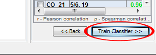
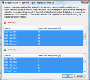
Generate Optimized Biomarker Models

Now, the optimization step follows, in which single CpG sites in the biomarkers get weights according to their "predictiveness". This is done with logistic regression models.

Click on "Train Classifier..." to start the process for checked biomarkers. MethMarker will now ask you for the training set used to train the classifiers. As default, MethMarker uses all loaded samples for training. If you want to exclude a specific sample, just deselect it. For this tutorial, accept all samples and press "OK".

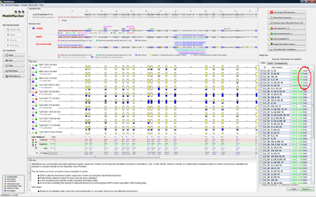
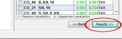
MethMarker has now created logistic regression models for checked biomarkers. This is indicated by a "calc." in the last column of the biomarker table. Biomarkers without regression models are labeled with "N/A".

Open the biomarker result window with click on "Results >>".

TIP: Alternatively, you can doubleclick on a biomarker with calculated logistic regression model in the biomarker table.

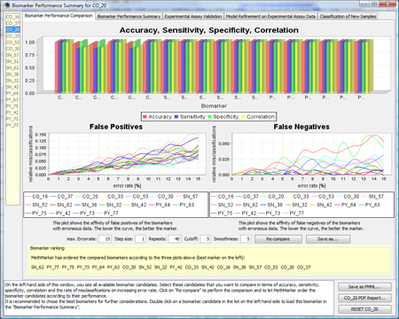
Now, you see the Biomarker Performance Summary, starting with the Biomarker Performance Comparison. The window is structured as follows:

• In the middle, all selected biomarkers (selected on the left) are compared to each other according to statistical accuracy, specitivity, sensitivity and correlation, FP rate and FN rate for errorneous data.
• On the left side, you can choose a biomarker from all available biomarkers. For this tutorial, doubleclick on CO_20 to choose biomarker candidate CO_20.
• On the bottom, there is an explanation of each biomarker performance summary window. Moreover, you can save here the biomarker result as PDF, or reset the biomarker if you have altered it.

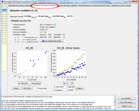
To get a more detailed overview about the biomarker, click on Biomarker Performance Summary on top of this window. Then, you get an overview of the statistical validation and Leave-One-Out Cross-Validation (with logistic regression formula, some performance data such as accuracy, specificity, sensitivity and correlation) and the experimental validation / classification. How the experimental classification can be used is explained in tutorial 2.

• The left one shows the classification of all loaded samples according to this biomarker candidate. MethMarker calculates the scores of the respective CpG sites (calculation is based on bisulfite sequenced samples), and computes the biomarker score for each sample. It correlates this score with the sample's overall methylation grade in this plot. A vertical line on 0 should separate methylated from unmethylated samples.
• The right plot shows how this biomarker candidate deals with errorneous data. A good biomarker should have low FN and FP rate even for relatively high error rates.

If you click on "Error Test", you can see how robustly the model behaves in the presence of erroneous data. For more information about the Error Test, look at the F.A.Q..

TIP: If you don't know how to interpret the regression formula, look at the F.A.Q..

TIP: If you don't know how to interpret accuracy, specificity, sensitivity or correlation, look at the F.A.Q..

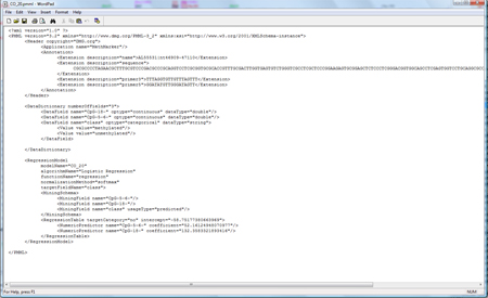
You can save the model as PMML file (press "Save CO_20 as..." on the right). A PMML file contains the model in a standardized statistical markup language, defined by the data mining group (http://www.dmg.org). Several statistical programms support PMML, and so does MethMarker.

For a comprehensive report of this biomarker candidate, click on "CO_20 PDF Report...". The PDF report is for your documents or can be shared with colleagues.

MethMarker has now created biomarkers, optimized with logistic regression model and validated with Leave-One-Out Cross-Validation. After saving the models (or saving the whole analysis with "File -> Save Analysis..."), you can close MethMarker.

<< back | next >>